Parallel computing

Parallel computing is a form of computation in which many calculations are carried out simultaneously, operating on the principle that large problems can often be divided into smaller ones, which are then solved concurrently ("in parallel"). There are several different forms of parallel computing: bit-level, instruction level, data, and task parallelism. Parallelism has been employed for many years, mainly in high-performance computing, but interest in it has grown lately due to the physical constraints preventing frequency scaling. As power consumption (and consequently heat generation) by computers has become a concern in recent years, parallel computing has become the dominant paradigm in computer architecture, mainly in the form of multicore processors.

Parallel computers can be roughly classified according to the level at which the hardware supports parallelism—with multi-core and multi-processor computers having multiple processing elements within a single machine, while clusters, MPPs, and grids use multiple computers to work on the same task. Specialized parallel computer architectures are sometimes used alongside traditional processors, for accelerating specific tasks.

Parallel computer programs are more difficult to write than sequential ones, because concurrency introduces several new classes of potential software bugs, of which race conditions are the most common. Communication and synchronization between the different subtasks are typically one of the greatest obstacles to getting good parallel program performance.

The speed-up of a program as a result of parallelization is governed by Amdahl's law.

Background

Traditionally, computer software has been written for serial computation. To solve a problem, an algorithm is constructed and implemented as a serial stream of instructions. These instructions are executed on a central processing unit on one computer. Only one instruction may execute at a time—after that instruction is finished, the next is executed.

Parallel computing, on the other hand, uses multiple processing elements simultaneously to solve a problem. This is accomplished by breaking the problem into independent parts so that each processing element can execute its part of the algorithm simultaneously with the others. The processing elements can be diverse and include resources such as a single computer with multiple processors, several networked computers, specialized hardware, or any combination of the above.

Frequency scaling was the dominant reason for improvements in computer performance from the mid-1980s until 2004. The runtime of a program is equal to the number of instructions multiplied by the average time per instruction. Maintaining everything else constant, increasing the clock frequency decreases the average time it takes to execute an instruction. An increase in frequency thus decreases runtime for all computation-bounded programs.

However, power consumption by a chip is given by the equation P = C × V² × F, where P is power, C is the capacitance being switched per clock cycle (proportional to the number of transistors whose inputs change), V is voltage, and F is the processor frequency (cycles per second).^[8] Increases in frequency increase the amount of power used in a processor. Increasing processor power consumption led ultimately to Intel's May 2004 cancellation of its Tejas and Jayhawk processors, which is generally cited as the end of frequency scaling as the dominant computer architecture paradigm.

Moore's Law is the empirical observation that transistor density in a microprocessor doubles every 18 to 24 months. Despite power consumption issues, and repeated predictions of its end, Moore's law is still in effect. With the end of frequency scaling, these additional transistors (which are no longer used for frequency scaling) can be used to add extra hardware for parallel computing.

Amdahl's law and Gustafson's law

A graphical representation of Amdahl's law. The speed-up of a program from parallelization is limited by how much of the program can be parallelized. For example, if 90% of the program can be parallelized, the theoretical maximum speed-up using parallel computing would be 10x no matter how many processors are used.

Optimally, the speed-up from parallelization would be linear—doubling the number of processing elements should halve the runtime, and doubling it a second time should again halve the runtime. However, very few parallel algorithms achieve optimal speed-up. Most of them have a near-linear speed-up for small numbers of processing elements, which flattens out into a constant value for large numbers of processing elements.

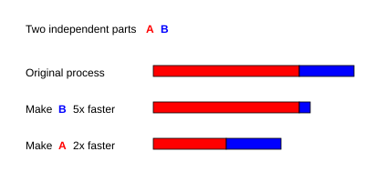
The potential speed-up of an algorithm on a parallel computing platform is given by Amdahl's law, originally formulated by Gene Amdahl in the 1960s. It states that a small portion of the program which cannot be parallelized will limit the overall speed-up available from parallelization. Any large mathematical or engineering problem will typically consist of several parallelizable parts and several non-parallelizable (sequential) parts. This relationship is given by the equation:

where S is the speed-up of the program (as a factor of its original sequential runtime), and P is the fraction that is parallelizable. If the sequential portion of a program is 10% of the runtime, we can get no more than a 10× speed-up, regardless of how many processors are added. This puts an upper limit on the usefulness of adding more parallel execution units. "When a task cannot be partitioned because of sequential constraints, the application of more effort has no effect on the schedule. The bearing of a child takes nine months, no matter how many women are assigned."

Gustafson's law is another law in computer engineering, closely related to Amdahl's law. It can be formulated as:

Assume that a task has two independent parts, A and B. B takes roughly 25% of the time of the whole computation. With effort, a programmer may be able to make this part five times faster, but this only reduces the time for the whole computation by a little. In contrast, one may need to perform less work to make part A twice as fast. This will make the computation much faster than by optimizing part B, even though B got a greater speed-up (5× versus 2×).

where P is the number of processors, S is the speed-up, and α the non-parallelizable part of the process. Amdahl's law assumes a fixed problem size and that the size of the sequential section is independent of the number of processors, whereas Gustafson's law does not make these assumptions.

Dependencies

Understanding data dependencies is fundamental in implementing parallel algorithms. No program can run more quickly than the longest chain of dependent calculations (known as the critical path), since calculations that depend upon prior calculations in the chain must be executed in order. However, most algorithms do not consist of just a long chain of dependent calculations; there are usually opportunities to execute independent calculations in parallel.

Let P_i and P_j be two program fragments. Bernstein's conditions describe when the two are independent and can be executed in parallel. For P_i, let I_i be all of the input variables and O_i the output variables, and likewise for P_j. P _i and P_j are independent if they satisfy

• 
• 
• 

Violation of the first condition introduces a flow dependency, corresponding to the first statement producing a result used by the second statement. The second condition represents an anti-dependency, when the first statement overwrites a variable needed by the second expression. The third and final condition represents an output dependency: When two statements write to the same location, the final result must come from the logically last executed statement.

Consider the following functions, which demonstrate several kinds of dependencies:

1: function Dep(a, b)
2:    c := a·b
3:    d := 2·c
4: end function

Operation 3 in Dep(a, b) cannot be executed before (or even in parallel with) operation 2, because operation 3 uses a result from operation 2. It violates condition 1, and thus introduces a flow dependency.

1: function NoDep(a, b)
2:      c := a·b
3:      d := 2·b
4:      e := a+b
5: end function

In this example, there are no dependencies between the instructions, so they can all be run in parallel.

Bernstein’s conditions do not allow memory to be shared between different processes. For that, some means of enforcing an ordering between accesses is necessary, such as semaphores, barriers or some other synchronization method.

Race conditions, mutual exclusion, synchronization, and parallel slowdown

Subtasks in a parallel program are often called threads. Some parallel computer architectures use smaller, lightweight versions of threads known as fibers, while others use bigger versions known as processes. However, "threads" is generally accepted as a generic term for subtasks. Threads will often need to update some variable that is shared between them. The instructions between the two programs may be interleaved in any order. For example, consider the following program:

Thread A	Thread B
1A: Read variable V	1B: Read variable V
2A: Add 1 to variable V	2B: Add 1 to variable V
3A Write back to variable V	3B: Write back to variable V

If instruction 1B is executed between 1A and 3A, or if instruction 1A is executed between 1B and 3B, the program will produce incorrect data. This is known as a race condition. The programmer must use a lock to provide mutual exclusion. A lock is a programming language construct that allows one thread to take control of a variable and prevent other threads from reading or writing it, until that variable is unlocked. The thread holding the lock is free to execute its critical section (the section of a program that requires exclusive access to some variable), and to unlock the data when it is finished. Therefore, to guarantee correct program execution, the above program can be rewritten to use locks:

Thread A	Thread B
1A: Lock variable V	1B: Lock variable V
2A: Read variable V	2B: Read variable V
3A: Add 1 to variable V	3B: Add 1 to variable V
4A Write back to variable V	4B: Write back to variable V
5A: Unlock variable V	5B: Unlock variable V

One thread will successfully lock variable V, while the other thread will be locked out—unable to proceed until V is unlocked again. This guarantees correct execution of the program. Locks, while necessary to ensure correct program execution, can greatly slow a program.

Locking multiple variables using non-atomic locks introduces the possibility of program deadlock. An atomic lock locks multiple variables all at once. If it cannot lock all of them, it does not lock any of them. If two threads each need to lock the same two variables using non-atomic locks, it is possible that one thread will lock one of them and the second thread will lock the second variable. In such a case, neither thread can complete, and deadlock results.

Many parallel programs require that their subtasks act in synchrony. This requires the use of a barrier. Barriers are typically implemented using a software lock. One class of algorithms, known as lock-free and wait-free algorithms, altogether avoids the use of locks and barriers. However, this approach is generally difficult to implement and requires correctly designed data structures.

Not all parallelization results in speed-up. Generally, as a task is split up into more and more threads, those threads spend an ever-increasing portion of their time communicating with each other. Eventually, the overhead from communication dominates the time spent solving the problem, and further parallelization (that is, splitting the workload over even more threads) increases rather than decreases the amount of time required to finish. This is known as parallel slowdown.

Fine-grained, coarse-grained, and embarrassing parallelism

Applications are often classified according to how often their subtasks need to synchronize or communicate with each other. An application exhibits fine-grained parallelism if its subtasks must communicate many times per second; it exhibits coarse-grained parallelism if they do not communicate many times per second, and it is embarrassingly parallel if they rarely or never have to communicate. Embarrassingly parallel applications are considered the easiest to parallelize.

Consistency models

Main article: Consistency model

Leslie Lamport first defined the concept of sequential consistency.

Parallel programming languages and parallel computers must have a consistency model (also known as a memory model). The consistency model defines rules for how operations on computer memory occur and how results are produced.

One of the first consistency models was Leslie Lamport's sequential consistency model. Sequential consistency is the property of a parallel program that its parallel execution produces the same results as a sequential program. Specifically, a program is sequentially consistent if "... the results of any execution is the same as if the operations of all the processors were executed in some sequential order, and the operations of each individual processor appear in this sequence in the order specified by its program".^[16]

Software transactional memory is a common type of consistency model. Software transactional memory borrows from database theory the concept of atomic transactions and applies them to memory accesses.

Mathematically, these models can be represented in several ways. Petri nets, which were introduced in Carl Adam Petri's 1962 doctoral thesis, were an early attempt to codify the rules of consistency models. Dataflow theory later built upon these, and Dataflow architectures were created to physically implement the ideas of dataflow theory. Beginning in the late 1970s, process calculi such as Calculus of Communicating Systems and Communicating Sequential Processes were developed to permit algebraic reasoning about systems composed of interacting components. More recent additions to the process calculus family, such as the π-calculus, have added the capability for reasoning about dynamic topologies. Logics such as Lamport's TLA+, and mathematical models such as traces and Actor event diagrams, have also been developed to describe the behavior of concurrent systems.

Flynn's taxonomy

Michael J. Flynn created one of the earliest classification systems for parallel (and sequential) computers and programs, now known as Flynn's taxonomy. Flynn classified programs and computers by whether they were operating using a single set or multiple sets of instructions, whether or not those instructions were using a single or multiple sets of data.

Flynn's taxonomy

	Single Instruction	Multiple Instruction
Single Data	SISD	MISD
Multiple Data	SIMD	MIMD
This box: view • talk • edit

The single-instruction-single-data (SISD) classification is equivalent to an entirely sequential program. The single-instruction-multiple-data (SIMD) classification is analogous to doing the same operation repeatedly over a large data set. This is commonly done in signal processing applications. Multiple-instruction-single-data (MISD) is a rarely used classification. While computer architectures to deal with this were devised (such as systolic arrays), few applications that fit this class materialized. Multiple-instruction-multiple-data (MIMD) programs are by far the most common type of parallel programs.

According to David A. Patterson and John L. Hennessy, "Some machines are hybrids of these categories, of course, but this classic model has survived because it is simple, easy to understand, and gives a good first approximation. It is also—perhaps because of its understandability—the most widely used scheme."

Types of parallelism

Bit-level parallelism

Main article: Bit-level parallelism

From the advent of very-large-scale integration (VLSI) computer-chip fabrication technology in the 1970s until about 1986, speed-up in computer architecture was driven by doubling computer word size—the amount of information the processor can manipulate per cycle. Increasing the word size reduces the number of instructions the processor must execute to perform an operation on variables whose sizes are greater than the length of the word. For example, where an 8-bit processor must add two 16-bit integers, the processor must first add the 8 lower-order bits from each integer using the standard addition instruction, then add the 8 higher-order bits using an add-with-carry instruction and the carry bit from the lower order addition; thus, an 8-bit processor requires two instructions to complete a single operation, where a 16-bit processor would be able to complete the operation with a single instruction.

Historically, 4-bit microprocessors were replaced with 8-bit, then 16-bit, then 32-bit microprocessors. This trend generally came to an end with the introduction of 32-bit processors, which has been a standard in general-purpose computing for two decades. Not until recently (c. 2003–2004), with the advent of x86-64 architectures, have 64-bit processors become commonplace.

Instruction-level parallelism

Main article: Instruction level parallelism

A canonical five-stage pipeline in a RISC machine (IF = Instruction Fetch, ID = Instruction Decode, EX = Execute, MEM = Memory access, WB = Register write back)

A computer program is, in essence, a stream of instructions executed by a processor. These instructions can be re-ordered and combined into groups which are then executed in parallel without changing the result of the program. This is known as instruction-level parallelism. Advances in instruction-level parallelism dominated computer architecture from the mid-1980s until the mid-1990s.

Modern processors have multi-stage instruction pipelines. Each stage in the pipeline corresponds to a different action the processor performs on that instruction in that stage; a processor with an N-stage pipeline can have up to N different instructions at different stages of completion. The canonical example of a pipelined processor is a RISC processor, with five stages: instruction fetch, decode, execute, memory access, and write back. The Pentium 4 processor had a 35-stage pipeline.

A five-stage pipelined superscalar processor, capable of issuing two instructions per cycle. It can have two instructions in each stage of the pipeline, for a total of up to 10 instructions (shown in green) being simultaneously executed.

In addition to instruction-level parallelism from pipelining, some processors can issue more than one instruction at a time. These are known as superscalar processors. Instructions can be grouped together only if there is no data dependency between them. Scoreboarding and the Tomasulo algorithm (which is similar to scoreboarding but makes use of register renaming) are two of the most common techniques for implementing out-of-order execution and instruction-level parallelism.

Data parallelism

Main article: Data parallelism

Data parallelism is parallelism inherent in program loops, which focuses on distributing the data across different computing nodes to be processed in parallel. "Parallelizing loops often leads to similar (not necessarily identical) operation sequences or functions being performed on elements of a large data structure." Many scientific and engineering applications exhibit data parallelism.

A loop-carried dependency is the dependence of a loop iteration on the output of one or more previous iterations. Loop-carried dependencies prevent the parallelization of loops. For example, consider the following pseudocode that computes the first few Fibonacci numbers:

1:    PREV1 := 0
2:    PREV2 := 1
4:    do:
5:       CUR := PREV1 + PREV2
6:       PREV1 := PREV2
7:       PREV2 := CUR
8:    while (CUR < 10)

This loop cannot be parallelized because CUR depends on itself (PREV2) and PREV1, which are computed in each loop iteration. Since each iteration depends on the result of the previous one, they cannot be performed in parallel. As the size of a problem gets bigger, the amount of data-parallelism available usually does as well.

Task parallelism

Main article: Task parallelism

Task parallelism is the characteristic of a parallel program that "entirely different calculations can be performed on either the same or different sets of data". This contrasts with data parallelism, where the same calculation is performed on the same or different sets of data. Task parallelism does not usually scale with the size of a problem.

Hardware

Memory and communication

Main memory in a parallel computer is either shared memory (shared between all processing elements in a single address space), or distributed memory (in which each processing element has its own local address space). Distributed memory refers to the fact that the memory is logically distributed, but often implies that it is physically distributed as well. Distributed shared memory and memory virtualization combine the two approaches, where the processing element has its own local memory and access to the memory on non-local processors. Accesses to local memory are typically faster than accesses to non-local memory.

A logical view of a Non-Uniform Memory Access (NUMA) architecture. Processors in one directory can access that directory's memory with less latency than they can access memory in the other directory's memory.

Computer architectures in which each element of main memory can be accessed with equal latency and bandwidth are known as Uniform Memory Access (UMA) systems. Typically, that can be achieved only by a shared memory system, in which the memory is not physically distributed. A system that does not have this property is known as a Non-Uniform Memory Access (NUMA) architecture. Distributed memory systems have non-uniform memory access.

Computer systems make use of caches—small, fast memories located close to the processor which store temporary copies of memory values (nearby in both the physical and logical sense). Parallel computer systems have difficulties with caches that may store the same value in more than one location, with the possibility of incorrect program execution. These computers require a cache coherency system, which keeps track of cached values and strategically purges them, thus ensuring correct program execution. Bus snooping is one of the most common methods for keeping track of which values are being accessed (and thus should be purged). Designing large, high-performance cache coherence systems is a very difficult problem in computer architecture. As a result, shared-memory computer architectures do not scale as well as distributed memory systems do.

Processor–processor and processor–memory communication can be implemented in hardware in several ways, including via shared (either multiported or multiplexed) memory, a crossbar switch, a shared bus or an interconnect network of a myriad of topologies including star, ring, tree, hypercube, fat hypercube (a hypercube with more than one processor at a node), or n-dimensional mesh.

Parallel computers based on interconnect networks need to have some kind of routing to enable the passing of messages between nodes that are not directly connected. The medium used for communication between the processors is likely to be hierarchical in large multiprocessor machines.

Classes of parallel computers

Parallel computers can be roughly classified according to the level at which the hardware supports parallelism. This classification is broadly analogous to the distance between basic computing nodes. These are not mutually exclusive; for example, clusters of symmetric multiprocessors are relatively common.

Multicore computing

Main article: Multi-core (computing)

A multicore processor is a processor that includes multiple execution units ("cores"). These processors differ from superscalar processors, which can issue multiple instructions per cycle from one instruction stream (thread); by contrast, a multicore processor can issue multiple instructions per cycle from multiple instruction streams. Each core in a multicore processor can potentially be superscalar as well—that is, on every cycle, each core can issue multiple instructions from one instruction stream.

Simultaneous multithreading (of which Intel's HyperThreading is the best known) was an early form of pseudo-multicoreism. A processor capable of simultaneous multithreading has only one execution unit ("core"), but when that execution unit is idling (such as during a cache miss), it uses that execution unit to process a second thread. IBM's Cell microprocessor, designed for use in the Sony Playstation 3, is another prominent multicore processor.

Symmetric multiprocessing

Main article: Symmetric multiprocessing

A symmetric multiprocessor (SMP) is a computer system with multiple identical processors that share memory and connect via a bus. Bus contention prevents bus architectures from scaling. As a result, SMPs generally do not comprise more than 32 processors. "Because of the small size of the processors and the significant reduction in the requirements for bus bandwidth achieved by large caches, such symmetric multiprocessors are extremely cost-effective, provided that a sufficient amount of memory bandwidth exists."

Distributed computing

Main article: Distributed computing

A distributed computer (also known as a distributed memory multiprocessor) is a distributed memory computer system in which the processing elements are connected by a network. Distributed computers are highly scalable.

Cluster computing

Main article: Computer cluster

A Beowulf cluster

A cluster is a group of loosely coupled computers that work together closely, so that in some respects they can be regarded as a single computer. Clusters are composed of multiple standalone machines connected by a network. While machines in a cluster do not have to be symmetric, load balancing is more difficult if they are not. The most common type of cluster is the Beowulf cluster, which is a cluster implemented on multiple identical commercial off-the-shelf computers connected with a TCP/IP Ethernet local area network.^[27] Beowulf technology was originally developed by Thomas Sterling and Donald Becker. The vast majority of the TOP500 supercomputers are clusters.

Massive parallel processing

Main article: Massive parallel processing

A massively parallel processor (MPP) is a single computer with many networked processors. MPPs have many of the same characteristics as clusters, but MPPs have specialized interconnect networks (whereas clusters use commodity hardware for networking). MPPs also tend to be larger than clusters, typically having "far more" than 100 processors. In an MPP, "each CPU contains its own memory and copy of the operating system and application. Each subsystem communicates with the others via a high-speed interconnect."

A cabinet from Blue Gene/L, ranked as the fourth fastest supercomputer in the world according to the 11/2008 TOP500 rankings. Blue Gene/L is a massively parallel processor.

Blue Gene/L, the fifth fastest supercomputer in the world according to the June 2009 TOP500 ranking, is an MPP.

Grid computing

Main article: Grid computing

Grid computing is the most distributed form of parallel computing. It makes use of computers communicating over the Internet to work on a given problem. Because of the low bandwidth and extremely high latency available on the Internet, grid computing typically deals only with embarrassingly parallel problems. Many grid computing applications have been created, of which SETI@home and Folding@Home are the best-known examples.

Most grid computing applications use middleware, software that sits between the operating system and the application to manage network resources and standardize the software interface. The most common grid computing middleware is the Berkeley Open Infrastructure for Network Computing (BOINC). Often, grid computing software makes use of "spare cycles", performing computations at times when a computer is idling.

Specialized parallel computers

Within parallel computing, there are specialized parallel devices that remain niche areas of interest. While not domain-specific, they tend to be applicable to only a few classes of parallel problems.

Reconfigurable computing with field-programmable gate arrays

Reconfigurable computing is the use of a field-programmable gate array (FPGA) as a co-processor to a general-purpose computer. An FPGA is, in essence, a computer chip that can rewire itself for a given task.

FPGAs can be programmed with hardware description languages such as VHDL or Verilog. However, programming in these languages can be tedious. Several vendors have created C to HDL languages that attempt to emulate the syntax and/or semantics of the C programming language, with which most programmers are familiar. The best known C to HDL languages are Mitrion-C, Impulse C, DIME-C, and Handel-C. Specific subsets of SystemC based on C++ can also be used for this purpose.

AMD's decision to open its HyperTransport technology to third-party vendors has become the enabling technology for high-performance reconfigurable computing. According to Michael R. D'Amour, Chief Operating Officer of DRC Computer Corporation, "when we first walked into AMD, they called us 'the socket stealers.' Now they call us their partners."

General-purpose computing on graphics processing units (GPGPU)

Main article: GPGPU

Nvidia's Tesla GPGPU card

General-purpose computing on graphics processing units (GPGPU) is a fairly recent trend in computer engineering research. GPUs are co-processors that have been heavily optimized for computer graphics processing. Computer graphics processing is a field dominated by data parallel operations—particularly linear algebra matrix operations.

In the early days, GPGPU programs used the normal graphics APIs for executing programs. However, recently several new programming languages and platforms have been built to do general purpose computation on GPUs with both Nvidia and AMD releasing programming environments with CUDA and CTM respectively. Other GPU programming languages are BrookGPU, PeakStream, and RapidMind. Nvidia has also released specific products for computation in their Tesla series.

Application-specific integrated circuits

Main article: Application-specific integrated circuit

Several application-specific integrated circuit (ASIC) approaches have been devised for dealing with parallel applications.^[34][35][36]

Because an ASIC is (by definition) specific to a given application, it can be fully optimized for that application. As a result, for a given application, an ASIC tends to outperform a general-purpose computer. However, ASICs are created by X-ray lithography. This process requires a mask, which can be extremely expensive. A single mask can cost over a million US dollars.^[37] (The smaller the transistors required for the chip, the more expensive the mask will be.) Meanwhile, performance increases in general-purpose computing over time (as described by Moore's Law) tend to wipe out these gains in only one or two chip generations. High initial cost, and the tendency to be overtaken by Moore's-law-driven general-purpose computing, has rendered ASICs unfeasible for most parallel computing applications. However, some have been built. One example is the peta-flop RIKEN MDGRAPE-3 machine which uses custom ASICs for molecular dynamics simulation.

Vector processors

Main article: Vector processor

The Cray-1 is the most famous vector processor.

A vector processor is a CPU or computer system that can execute the same instruction on large sets of data. "Vector processors have high-level operations that work on linear arrays of numbers or vectors. An example vector operation is A = B × C, where A, B, and C are each 64-element vectors of 64-bit floating-point numbers." They are closely related to Flynn's SIMD classification.

Cray computers became famous for their vector-processing computers in the 1970s and 1980s. However, vector processors—both as CPUs and as full computer systems—have generally disappeared. Modern processor instruction sets do include some vector processing instructions, such as with AltiVec and Streaming SIMD Extensions (SSE).

Software

Parallel programming languages

Main article: parallel programming model

Concurrent programming languages, libraries, APIs, and parallel programming models have been created for programming parallel computers. These can generally be divided into classes based on the assumptions they make about the underlying memory architecture—shared memory, distributed memory, or shared distributed memory. Shared memory programming languages communicate by manipulating shared memory variables. Distributed memory uses message passing. POSIX Threads and OpenMP are two of most widely used shared memory APIs, whereas Message Passing Interface (MPI) is the most widely used message-passing system API. One concept used in programming parallel programs is the future concept, where one part of a program promises to deliver a required datum to another part of a program at some future time.

Automatic parallelization

Main article: Automatic parallelization

Automatic parallelization of a sequential program by a compiler is the holy grail of parallel computing. Despite decades of work by compiler researchers, automatic parallelization has had only limited success.

Mainstream parallel programming languages remain either explicitly parallel or (at best) partially implicit, in which a programmer gives the compiler directives for parallelization. A few fully implicit parallel programming languages exist—SISAL, Parallel Haskell, and (for FPGAs) Mitrion-C.

Application checkpointing

Main article: Application checkpointing

The larger and more complex a computer is, the more that can go wrong and the shorter the mean time between failures. Application checkpointing is a technique whereby the computer system takes a "snapshot" of the application—a record of all current resource allocations and variable states, akin to a core dump; this information can be used to restore the program if the computer should fail. Application checkpointing means that the program has to restart from only its last checkpoint rather than the beginning. For an application that may run for months, that is critical. Application checkpointing may be used to facilitate process migration.

Applications

As parallel computers become larger and faster, it becomes feasible to solve problems that previously took too long to run. Parallel computing is used in a wide range of fields, from bioinformatics (to do protein folding) to economics (to do simulation in mathematical finance). Common types of problems found in parallel computing applications are:

• Dense linear algebra
• Sparse linear algebra
• Spectral methods (such as Cooley–Tukey fast Fourier transform)
• N-body problems (such as Barnes-Hut simulation)
• Structured grid problems (such as Lattice Boltzmann methods)
• Unstructured grid problems (such as found in finite element analysis)
• Monte Carlo simulation
• Combinational logic (such as brute-force cryptographic techniques)
• Graph traversal (such as sorting algorithms)
• Dynamic programming
• Branch and bound methods
• Graphical models (such as detecting hidden Markov models and constructing Bayesian networks)
• Finite-state machine simulation

History

Main article: History of computing

ILLIAC IV, "perhaps the most infamous of Supercomputers"

The origins of true (MIMD) parallelism go back to Federico Luigi, Conte Menabrea and his "Sketch of the Analytic Engine Invented by Charles Babbage". IBM introduced the 704 in 1954, through a project in which Gene Amdahl was one of the principal architects. It became the first commercially available computer to use fully automatic floating point arithmetic commands.

In April 1958, S. Gill (Ferranti) discussed parallel programming and the need for branching and waiting. Also in 1958, IBM researchers John Cocke and Daniel Slotnick discussed the use of parallelism in numerical calculations for the first time. Burroughs Corporation introduced the D825 in 1962, a four-processor computer that accessed up to 16 memory modules through a crossbar switch. In 1967, Amdahl and Slotnick published a debate about the feasibility of parallel processing at American Federation of Information Processing Societies Conference. It was during this debate that Amdahl's Law was coined to define the limit of speed-up due to parallelism.

In 1969, US company Honeywell introduced its first Multics system, a symmetric multiprocessor system capable of running up to eight processors in parallel.^[46] C.mmp, a 1970s multi-processor project at Carnegie Mellon University, was "among the first multiprocessors with more than a few processors". "The first bus-connected multi-processor with snooping caches was the Synapse N+1 in 1984."

SIMD parallel computers can be traced back to the 1970s. The motivation behind early SIMD computers was to amortize the gate delay of the processor's control unit over multiple instructions. In 1964, Slotnick had proposed building a massively parallel computer for the Lawrence Livermore National Laboratory. His design was funded by the US Air Force, which was the earliest SIMD parallel-computing effort, ILLIAC IV.^[46] The key to its design was a fairly high parallelism, with up to 256 processors, which allowed the machine to work on large datasets in what would later be known as vector processing. However, ILLIAC IV was called "the most infamous of Supercomputers", because the project was only one fourth completed, but took 11 years and cost almost four times the original estimate. When it was finally ready to run its first real application in 1976, it was outperformed by existing commercial supercomputers such as the Cray-1.

Binary search algorithm

In computer science, a binary search is an algorithm for locating the position of an element in a sorted list. It inspects the middle element of the sorted list: if equal to the sought value, then the position has been found; otherwise, the upper half or lower half is chosen for further searching based on whether the sought value is greater than or less than the middle element. The method reduces the number of elements needed to be checked by a factor of two each time, and finds the sought value if it exists in the list or if not determines "not present", in logarithmic time. A binary search is a dichotomic divide and conquer search algorithm.

Viewing the comparison as a subtraction of the sought value from the middle element, only the sign of the difference is inspected: there is no attempt at an interpolation search based on the size of the difference.

Overview

Finding the index of a specific value in a sorted list is useful because, given the index, other data structures will contain associated information. Suppose a data structure containing the classic collection of name, address, telephone number and so forth has been accumulated, and an array is prepared containing the names, numbered from one to N. A query might be: what is the telephone number for a given name X. To answer this the array would be searched and the index (if any) corresponding to that name determined, whereupon the associated telephone number array would have X's telephone number at that index, and likewise the address array and so forth. Appropriate provision must be made for the name not being in the list (typically by returning an index value of zero), indeed the question of interest might be only whether X is in the list or not.

If the list of names is in sorted order, a binary search will find a given name with far fewer probes than the simple procedure of probing each name in the list, one after the other in a linear search, and the procedure is much simpler than organizing a hash table. However, once created, searching with a hash table may well be faster, typically averaging just over one probe per lookup. With a non-uniform distribution of values, if it is known that some few items are much more likely to be sought for than the majority, then a linear search with the list ordered so that the most popular items are first may do better than binary search. The choice of the best method may not be immediately obvious. If, between searches, items in the list are modified or items are added or removed, maintaining the required organisation may consume more time than the searches.

Examples

Number guessing game

This rather simple game begins something like "I'm thinking of an integer between forty and sixty inclusive, and to your guesses I'll respond 'High', 'Low', or 'Yes!' as might be the case." Supposing that N is the number of possible values (here, twenty-one as "inclusive" was stated), then at most questions are required to determine the number, since each question halves the search space. Note that one less question (iteration) is required than for the general algorithm, since the number is already constrained to be within a particular range.

Even if the number we're guessing can be arbitrarily large, in which case there is no upper bound N, we can still find the number in at most steps (where k is the (unknown) selected number) by first finding an upper bound by repeated doubling.^{[citation needed]} For example, if the number were 11, we could use the following sequence of guesses to find it: 1, 2, 4, 8, 16, 12, 10, 11

One could also extend the technique to include negative numbers; for example the following guesses could be used to find −13: 0, −1, −2, −4, −8, −16, −12, −14, −13

Word lists

People typically use a mixture of the binary search and interpolative search algorithms when searching a telephone book, after the initial guess we exploit the fact that the entries are sorted and can rapidly find the required entry. For example when searching for Smith, if Rogers and Thomas have been found, one can flip to a page about halfway between the previous guesses. If this shows Samson, we know that Smith is somewhere between the Samson and Thomas pages so we can bisect these.

Applications to complexity theory

Even if we do not know a fixed range the number k falls in, we can still determine its value by asking simple yes/no questions of the form "Is k greater than x?" for some number x. As a simple consequence of this, if you can answer the question "Is this integer property k greater than a given value?" in some amount of time then you can find the value of that property in the same amount of time with an added factor of log₂k. This is called a reduction, and it is because of this kind of reduction that most complexity theorists concentrate on decision problems, algorithms that produce a simple yes/no answer.

For example, suppose we could answer "Does this n x n matrix have determinant larger than k?" in O(n²) time. Then, by using binary search, we could find the (ceiling of the) determinant itself in O(n²log d) time, where d is the determinant; notice that d is not the size of the input, but the size of the output.

The method

In order to discuss the method in detail, a more formal description is necessary. The basic idea is that there is a data structure represented by array A in which individual elements are identified as A(1), A(2),…,A(N) and may be accessed in any order. The data structure contains a sub-element or data field called here Key, and the array is ordered so that the successive values A(1).Key ≤ A(2).Key and so on. The requirement is that given some value x, find an index p (not necessarily the one and only) such that A(p).Key = x.

To begin with, the span to be searched is the full supplied list of elements, as marked by variables L and R, and their values are changed with each iteration of the search process, as depicted by the flowchart. Note that the division by two is integer division, with any remainder lost, so that 3/2 comes out as 1, not 1½. The search finishes either because the value has been found, or else, the specified value is not in the list.

That it works

The method relies on and upholds the notion If x is to be found, it will be amongst elements (L + 1) to (R − 1) of the array.

The initialisation of L and R to 0 and N + 1 make this merely a restatement of the supplied problem, that elements 1 to N are to be searched, so the notion is established to begin with. The first step of each iteration is to check that there is something to search, which is to say whether there are any elements in the search span (L + 1) to (R − 1). The number of such elements is (R − L − 1) so computing (R − L) gives (number of elements + 1); halving that number (with integer division) means that if there was one element (or more) then p = 1 (or more), but if none p = 0, and in that case the method terminates with the report "Not found". Otherwise, for p 0, the search continues with p:=L + p, which by construction is within the bounds (L + 1) to (R − 1). That this position is at or adjacent to the middle of the span is not important here, merely that it is a valid choice.

Now compare x to A(p).Key. If x = A(p).Key then the method terminates in success. Otherwise, suppose x . If so, then because the array is in sorted order, x will also be less than all later elements of the array, all the way to element (R − 1) as well. Accordingly, the value of the right-hand bound index R can be changed to be the value p, since, by the test just made, x and so, if x is to be found, it will be amongst elements earlier than p, that is (p − 1) and earlier. And contrariwise, for the case x A(p).Key, the value of L would be changed. Thus, whichever bound is changed the ruling notion is upheld, and further, the span remaining to be searched is reduced. If L is changed, it is changed to a higher number (at least L + 1), whereas if R is changed, it is to a lower number (at most R − 1) because those are the limits for p.

Should there have been just one value remaining in the search span (so that L + 1 = p = R − 1), and x did not match, then depending on the sign of the comparison either L or R will receive the value of p and at the start of the next iteration the span will be found to be empty.

Accordingly, with each iteration, if the search span is empty the result is "Not found", otherwise either x is found at the probe point p or the search span is reduced for the next iteration. Thus the method works, and so can be called an Algorithm.

That it is fast

With each iteration that fails to find a match at the probed position, the search is continued with one or other of the two sub-intervals, each at most half the size. More precisely, if the number of items, N, is odd then both sub-intervals will contain (N - 1)/2 elements. If N is even then the two sub-intervals contain N/2 - 1 and N/2 elements.

If the original number of items is N then after the first iteration there will be at most N/2 items remaining, then at most N/4 items, at most N/8 items, and so on. In the worst case, when the value is not in the list, the algorithm must continue iterating until the span has been made empty; this will have taken at most ⌊log₂(N) + 1⌋ iterations, where the ⌊ ⌋ notation denotes the floor function that rounds its argument down to an integer. This worst case analysis is tight: for any N there exists a query that takes exactly ⌊log₂(N) + 1⌋ iterations. When compared to linear search, whose worst-case behaviour is N iterations, we see that binary search is substantially faster as N grows large. For example, to search a list of 1 million items takes as much as 1 million iterations with linear search, but never more than 20 iterations with binary search. However, binary search is only valid if the list is in sorted order.

Average performance

There are two cases: for searches that will fail because the value is not in the list, the search span must be successively halved until no more elements remain and this process will require at most the p probes just defined, or one less. This latter occurs because the search span is not in fact exactly halved, and depending on the value of N and which elements of the list the absent value x is between, the span may be closed early.

For searches that will succeed because the value is in the list, the search may finish early because a probed value happens to match. Loosely speaking, half the time the search will finish one iteration short of the maximum and a quarter of the time, two early. Consider then a test in which a list of N elements is searched once for each of the N values in the list, and determine the number of probes n for all N searches.

  N =  1   2    3    4     5     6     7     8     9    10     11     12     13
n/N =  1  3/2  5/3  8/4  11/5  14/6  17/7  21/8  25/9  29/10  33/11  37/12  41/13
   1  1.5  1.66  2    2.2  2.33  2.43  2.63  2.78   2.9    3     3.08   3.15

In short log₂(N) − 1 is about the expected number of probes in an average successful search, and the worst case is log₂(N), just one more probe. If the list is empty, no probes at all are made.

Suppose the list to be searched contains N even numbers (say, 2,4,6,8 for N = 4) and a search is done for values 1, 2, 3, 4, 5, 6, 7, 8, and 9. The even numbers will be found, and the average number of iterations can be calculated as described. In the case of the odd numbers, they will not be found, and the collection of test values probes every possible position (with regard to the numbers that are in the list) that they might be not found in, and an average is calculated. The maximum value is for each N the greatest number of iterations that were required amongst the various trail searches of those N elements. The first plot shows the iteration counts for N = 1 to 63 (with N = 1, all results are 1), and the second plot is for N = 1 to 32767.

Iteration count for 1 N

The curve for the "found" searches approaches log₂(N) − 1 more closely for larger N as larger numbers of iterations are involved, in the same way that the successive summations 1/2, 1/4 + 1/2, 1/8 + 1/4 + 1/2 approach 1 as the number of terms increases: these are the probabilities of early detection of equality in successive iterations of a search. The slight bend in the curves within each iteration limit group is due to the early narrowing of the search bounds into two sub-spans whose lengths are often unequal.

Iteration count for 1 N

Thus binary search is a logarithmic algorithm and executes in O(logN) time. In most cases it is considerably faster than a linear search. It can be implemented using iteration (as shown above), or recursion. In some languages it is more elegantly expressed recursively; however, in some C-based languages tail recursion is not eliminated and the recursive version requires more stack space.

Binary search can interact poorly with the memory hierarchy (i.e. caching), because of its random-access nature. For in-memory searching, if the span to be searched is small, a linear search may have superior performance simply because it exhibits better locality of reference. For external searching, care must be taken or each of the first several probes will lead to a disk seek. A common technique is to abandon binary searching for linear searching as soon as the size of the remaining span falls below a small value such as 8 or 16 or even more in recent computers. The exact value depends entirely on the machine running the algorithm.

Notice that for multiple searches with a fixed value for N, then (with the appropriate regard for integer division), the first iteration always selects the middle element at N/2, and the second always selects either N/4 or 3N/4, and so on. Thus if the array's key values are in some sort of slow storage (on a disc file, in virtual memory, not in the cpu's on-chip memory), keeping those three keys in a local array for a special preliminary search will avoid accessing widely separated memory. Escalating to seven or fifteen such values will allow further levels at not much cost in storage. On the other hand, if the searches are frequent and not separated by much other activity, the computer's various storage control features will more or less automatically promote frequently-accessed elements into faster storage.

When multiple binary searches are to be performed for the same key in related lists, fractional cascading can be used to speed up successive searches after the first one.

Extensions

There is no particular requirement that the array being searched has the bounds 1 to N. It is possible to search a specified range, elements first to last instead of 1 to N. All that is necessary is that the initialisation be L:=first − 1 and R:=last + 1, then all proceeds as before.

The elements of the list are not necessarily all unique. If one searches for a value that occurs multiple times in the list, the index returned will be of the first-encountered equal element, and this will not necessarily be that of the first, last, or middle element of the run of equal-key elements but will depend on the positions of the values. Modifying the list even in seemingly unrelated ways such as adding elements elsewhere in the list may change the result. To find all equal elements an upward and downward linear search can be carried out from the initial result, stopping each search when the element is no longer equal. Thus, e.g. in a table of cities sorted by country, we can find all cities in a given country.

Several algorithms closely related to or extending binary search exist. For instance, noisy binary search solves the same class of projects as regular binary search, with the added complexity that any given test can return a false value at random. (Usually, the number of such erroneous results are bounded in some way, either in the form of an average error rate, or in the total number of errors allowed per element in the search space.) Optimal algorithms for several classes of noisy binary search problems have been known since the late seventies, and more recently, optimal algorithms for noisy binary search in quantum computers (where several elements can be tested at the same time) have been discovered.

Variations

There are many, and they are easily confused.

Exclusive or inclusive bounds

The most significant differences are between the "exclusive" and "inclusive" forms of the bounds. This description uses the "exclusive" bound form, that is the span to be searched is (L + 1) to (R − 1), and this may seem clumsy when the span to be searched could be described in the "inclusive" form, as L to R. Although the details differ the two forms are equivalent as can be seen by transforming one version into the other. The inclusive bound form may be attained by replacing all appearances of "L" by "(L − 1)" and "R" by "(R + 1)" then rearranging. Thus, the initialisation of L:=0 becomes (L − 1):=0 or L:=1, and R:=N + 1 becomes (R + 1):=N + 1 or R:=N. So far so good, but note now that the changes to L and R are no longer simply transferring the value of p to L or R as appropriate but now must be (R + 1):=p or R:=p − 1, and (L − 1):=p or L:=p + 1.

Thus, the gain of a simpler initialisation, done once, is lost by a more complex calculation, and which is done for every iteration. If that is not enough, the test for an empty span is more complex also, as compared to the simplicity of checking that the value of p is zero. Nevertheless, the inclusive bound form is found in many publications, such as Donald Knuth. The Art of Computer Programming, Volume 3: Sorting and Searching, Third Edition.

Deferred detection of equality

Because of the syntax difficulties discussed below, so that distinguishing the three states , =, and would have to be done with two comparisons, it is possible to use just one comparison and at the end when the span is reduced to zero, equality can be tested for. The example distinguishes only from =.

Midpoint and width

An entirely different variation involves abandoning the L and R pointers in favour of a current position p and a width w where at each iteration, p is adjusted by + or − w and w is halved. Professor Knuth remarks "It is possible to do this, but only if extreme care is paid to the details" – Section 6.2.1, page 414 of The Art of Computer Programming, Volume 3: Sorting and Searching, Third Edition, outlines an algorithm, with the further remark "Simpler approaches are doomed to failure!"

Computer usage

The algorithm

"Although the basic idea of binary search is comparatively straightforward, the details can be surprisingly tricky…" — Professor Donald Knuth

When Jon Bentley assigned it as a problem in a course for professional programmers, he found that an astounding ninety percent failed to code a binary search correctly after several hours of working on it^[3], and another study shows that accurate code for it is only found in five out of twenty textbooks (Kruse, 1999). Furthermore, Bentley's own implementation of binary search, published in his 1986 book Programming Pearls, contains an error that remained undetected for over twenty years.

Numerical difficulties

In a practical implementation, the variables used to represent the indices will be of finite size, hence only capable of representing a finite range of values. For example, 16-bit unsigned integers can only hold values from 0 to 65535. If the binary search algorithm is to operate on large arrays, this has two implications:

• The values first − 1 and last + 1 must both be representable within the finite bounds of the chosen integer type . Therefore, continuing the 16-bit example, the largest value that last may take is +65534, not +65535. A problem exists even for the "inclusive" form of the method, as if x A(65535).Key, then on the final iteration the algorithm will attempt to store 65536 into L and fail. Equivalent issues apply to the lower limit (where first − 1 could become negative when the allowed search space only contains positive or null indice).
• If the midpoint of the span is calculated as p := (L + R) / 2, then the value (L + R) will exceed the number range if last is greater than (in our example) 65535/2 and the search wanders toward the upper end of the search space. This can be avoided by performing the calculation as p := L + (R - L) / 2.

Syntax difficulties

Another difficulty is presented by the absence in most computer languages of a three-way result from a comparison, which forces a comparison to be performed twice. The form is somewhat as follows:

if a 

About half the time, the first test will be true so that there will be only one comparison of a and b, but the other half of the time it will be false, and a second comparison forced. This is so grievous that some versions are recast so as not to make a second test at all thus not determining equality until the span has been reduced to zero, and thereby foregoing the possibility of early termination – remember that about half the time the search will happen on a matching value one iteration short of the limit.

It is quite easy to make this problem still worse (e.g. as in ^[5]) by using an order such as

if a = b then action3
else if a  b then action2
else action1;

Rather than detecting equality early (as it might appear to), this will force two comparisons to be performed for all but the last iteration of a search.

Implementations

Iterative

Niklaus Wirth recorded this algorithm in Standard Pascal ^[6] :

  min := 1;
max := N; {array size: var A : array [1..N] of integer}
repeat
mid := (min + max) div 2;
if x  A[mid] then
  min := mid + 1
else
  max := mid - 1;
until (A[mid] = x) or (min  max);

This code uses inclusive bounds and a three-way test (for early loop termination in case of equality), but with two separate comparisons per iteration. It is not the most efficient solution.

Three-way comparison

This section does not cite any references or sources. Please help improve this article by adding citations to reliable sources. Unsourced material may be challenged and removed. (January 2009)

Since Fortran does offer a three-way test, here is a version for searching an array of integers. For labels Fortran uses numbers at the start of statements, thus the 1, 2, 3, and 4. The if statement performs a go to to one of the three nominated labels according to the sign of its arithmetic expression.

      Integer Function BinarySearch(A,X,N)
  ! Search for the value X in A(1)..A(N)  
   Integer A(*),X          !The array is indexed 1 to ?     
   Integer N               !Stated number of elements.           
   Integer L,R,P
    L = 0                  !Exclusive bounds,
    R = N + 1              !To search elements 1 to N.
1   P = (R - L)/2          !Probe; integer division. Not (L + R)/2!
    if (P = 0) Return(-L) !Search exhausted.        P = L + P              !Convert an offset from L to an array index.        if (X - A(P)) 3,4,2    !Test: negative,zero,positive.    2   L = P                  !A(P) < r =" P" x =" A(P).">

Recursive

This section does not cite any references or sources. Please help improve this article by adding citations to reliable sources. Unsourced material may be challenged and removed. (January 2009)

The most straightforward implementation is recursive, which recursively searches the subrange dictated by the comparison:

   BinarySearch(A[0..N-1], value, low, high) {
   if (high  mid =" low" value)
       return BinarySearch(A, value, low, mid-1)
   else if (A[mid] 

It is invoked with initial low and high values of 0 and N-1. We can eliminate the tail recursion above and convert this to an iterative implementation:

Single comparison per iteration

This section does not cite any references or sources. Please help improve this article by adding citations to reliable sources. Unsourced material may be challenged and removed. (January 2009)

In computer languages that lack a three-way comparison, the required three-way comparison has to be replaced by two two-way comparisons that would on average involve one and a half comparisons per iteration, not one. To reduce this overhead, some implementations defer checking for equality until after the search completes, as in this pseudocode:

       low = 0
   high = N
   while (low  mid =" low" low =" mid" high =" mid-1:"= value,
            //so high can't be high =" mid;" high ="=""

This approach foregoes the possibility of early termination on discovery of a match, thus successful searches have log₂(N) iterations instead of an expected log₂(N) − 1 iterations. On the other hand, this implementation makes fewer comparisons: log₂(N) is less than the expected number of comparisons for the two-test implementations of 1·5(log₂(N) − 1), for N greater than eight.